Contents

1 Introduction

Bacteriophages are characterized by extreme mosaicism. Since mostly co-linearly ordered modules contain different variants that have very little sequence similarity, traditional multiple alignments are not appropriate for bacteriophage genomes.

Alpha is a browser designed for detailed comparative studies of bacteriophage genomes. It provides a convenient way to compute and view the partial order induced by exact matches¹ .

This document describes how to use Alpha in this context, providing tips for the novice user. The tool is introduced in [1]. Please reference it if you use Alpha in your research.

The workflow followed by a typical user interested in studying a set of phage genomes is the following:

1. Create a fasta file containing the genomes of interest.
2. Launch an interactive session by clicking the alpha icon, or by using the alpha command in the terminal.

These steps will be described in the coming sections. First, we show how to install the software under Ubuntu Linux and macOS.

• Please cite us [1] if you use Alpha in your work:
  Sèverine Bérard, Annie Chateau, Nicolas Pompidor, Paul Guertin, Anne Bergeron, and Krister M. Swenson. Aligning the unalignable: bacteriophage whole genome alignments. BMC Bioinformatics, 17(1):30, 2016.
• The code is hosted at https://bitbucket.org/thekswenson/alpha.

2 Installation

These are the instructions for easy installation under Ubuntu or macOS. Refer to the wiki for detailed instruction on installing Alpha if you are using another Linux distribution or a version of macOS older than High-Sierra.

2.1 Easy installation for Ubuntu

We have a PPA for easy installation and updates of Alpha. To install alpha run the following commands in a terminal:

1. “sudo add-apt-repository universe”
2. “sudo add-apt-repository ppa:thekswenson/alpha-aligner”
3. “sudo apt update”
4. “sudo apt install alpha-aligner”

2.2 Easy installation for macOS

These instructions will work for macOS 10.13 High-Sierra and later:

1. Download the .dmg file.
2. Double-click it.
3. Drag the Alpha icon into the application folder.

3 Using Alpha

Alpha is a tool for looking at common sequence structure in a set of phages. In general the tool can be used in two ways: 1) for focused study of an area of interest or 2) for browsing larger structure in the multiple alignment.

3.1 Overview

When launching Alpha, the first thing you see is the file loading dialog.

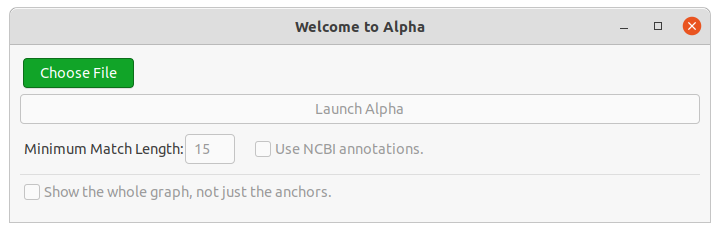
Choose a .fasta file or a saved .alpha to open. The genomes will then be loaded into the dialog (see Figure 1).

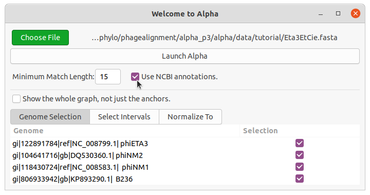
Make your desired configuration and then click “Launch Alpha”.

3.1.1 Anchor Mode

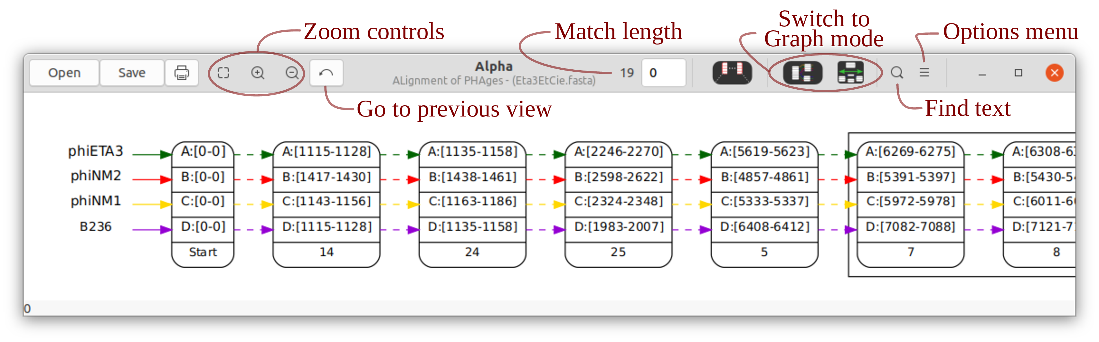
Unless the “Show the whole graph” box is checked, Alpha is opened in anchor mode. An anchor is a node corresponding to a perfect (i.e. all columns are identical) alignment that includes all input genomes. The initial window displays a graph with some of the anchors (see Figure 2). The boxes around the nodes indicate that some anchors have been omitted from the display between those anchors.

The purpose of the anchor view is to allow the user to target parts of the alignment while avoiding the costly step of computing the graph over the entire genome. You can focus on an area of the genome by highlighting two nodes and then clicking the “entry” button (hotkey Enter). This will show more anchors.

Anchor mode is finished when either the “contracted graph” button (hotkeys g, G) or the “expanded graph” button (hotkeys e, E) is pressed. The only way to return to anchor mode is to go back using the “back” button (hotkey Delete/Backspace or middle-click).

3.1.2 Browsing Basics

Use the mouse to move the image. Zoom with the mouse wheel. Select nodes by clicking on them. A selected node has a target in the upper-right corner that gives access to a menu. Hover the mouse over a button to see the hotkey and description of the button. A reference to the UI elements appears in Section 3.4.

See more detail for a specific part of the graph by highlighting two nodes and pressing the the “entry” button (hotkey Enter). Exit anchor mode by pressing the “contracted graph” button (hotkeys g, G) or the “expanded graph” button (hotkeys e, E). The views are stored in a stack, where previous graphs can be viewed using the “back” button (hotkey Delete/Backspace or middle-click).

3.1.3 Node Menus: Annotations, Alignments and Indices

When a node is highlighted, a menu is accessible by clicking on the red target that appears on the corner of the node. This menu contains different entries depending the identity of, and how many (1 or 2) nodes are highlighted. The potential entries are the following:

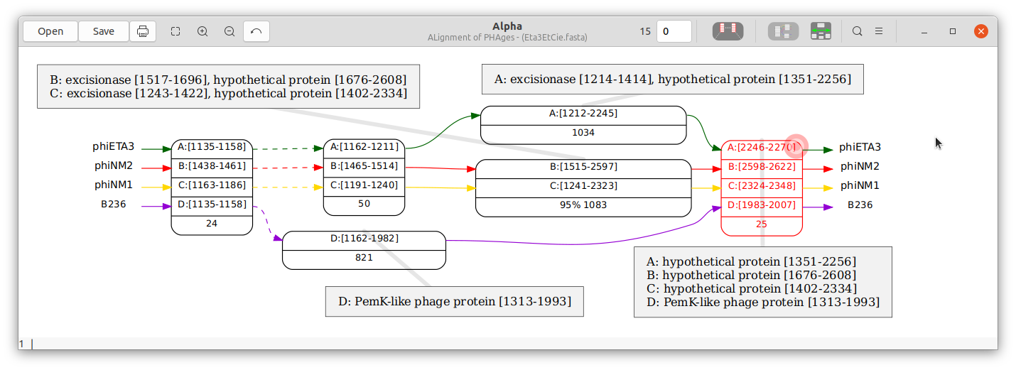
The annotations in the following example show that there is a “PemK-like protein” that shares 10 bases (the right-most node) with “hypothetical proteins” despite having very few exact matches within the preceding 600+ bases of the protein.

3.2 Tutorial

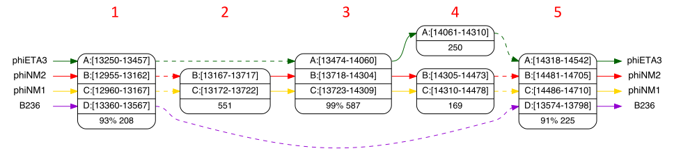
Say we would like to compare the region of phage phiNM2 between nucleotides 13000 and 14500 with the homologous regions in phiETA3, phiNM1, and B236. Download Eta3EtCie.fasta to get started. Launch Alpha and choose the file you just downloaded. You will see the screen from Figure 1. Press the “Launch Alpha” button.

You will see a linear ordering of a sampling of all anchors. phiNM2 is genome B. We’re interested in the interval B:[13000-14500] so click on the node with interval B:[12955-12970] and the node with interval B:[14691-14705] so that our desired interval will be include in the next view. Now click on the “contracted graph” button (hotkeys g, G). The result will look like Figure 3. We can see that there have been significant insertions/deletions that distinguish phiNM1 and phiNM2 from the other strains. Select the “Show Small Nodes” menu item (hotkey s) to view the minor differences between the strains. Select it again to hide them.

An alternate method to focus on this part of the alignment would be to load the fasta file, and choose the “Select Intervals” tab. Press the “Open” button (hotkey Ctrl-o) in the top left corner. You will see this after you have entered the intervals:

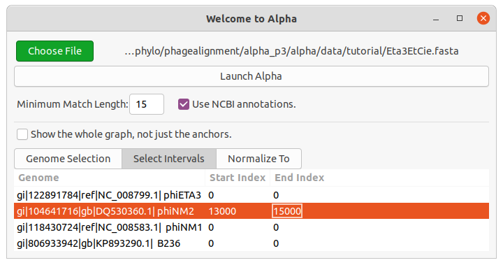
Alpha will now only process the chosen interval when you press “Launch Alpha”. Close the new window you just created.

3.2.1 Multiple Windows and CPUs

The computation of some graphs can take minutes. While a single graph will be computed on a single CPU, the inconvenience of waiting can be avoided by computing the next graph on a new CPU, opening the result in a new window. This way, the current view can continue to be explored while the new graph is being computed. To compute the next view in a new window either

• activate the “Open in New Window” menu item (hotkey n) before clicking one of the three graph buttons, or
• press Shift when using the hotkeys Enter, G, or E.

To try this feature, open a second window again with the “Open” button (hotkey Ctrl-o) and launch a new Alpha instance with the same input file. Highlight the nodes B:[36914-37018] and B:[40503-40566] and then activate the “Open in New Window” menu item (hotkey n), before clicking the “contracted graph” button (hotkeys g, G). See that a new window is opened once the computations have finished. You can close these two windows now.

3.2.2 Advanced exploration

Now we will play with the match length to get a finer resolution version of the same genomic area. Go to you primary window and click on the match entry box (hotkey m) and enter 8. Press the “entry” button (hotkey Enter). Alpha will recompute a graph, trying a minimum match length of 8. The match length 8 is so short, though, that there are multiple matches of that length for the same nucleotides, creating a cycle in the graph. Alpha now automatically tries larger match lengths and finds that 11 creates an acyclic graph. The large center node in column 3 has grown while the differences between phiETA3 and phiNM1/phiNM2 in column 4 have shrunk.

To see the cycle caused by the multiple length-8 matches, press the “back” button (hotkey Delete/Backspace or middle-click) and then enter 8 in the match entry box (hotkey m) again. This time, press the “expanded graph” button (hotkeys e, E). You will see the full graph, including the cycle. It turns out that there is an 8bp match between phiNM1/phiNM2 and phiETA3 just before the interval B:[13272-13320] that leads to the cycle.

3.3 General Exploration of a Multiple Alignment

We will explore the same dataset by viewing the graph in its entirety. In the welcome dialog, activate the “Show the whole graph” item. Note that this process can take a while, and that the resulting graph will have many nodes! To calibrate the size of the graph, we can specify a longer match length in the “Minimum Match Length” box. Enter 35 in that box and press “Launch Alpha”.

The result is a large graph (partial order) that you can browse for interesting features. At the interval between nodes A:[9130-9164] and A:[11574-11608] we see an interesting region where B236 (genome D) has a different variant from the others (hint: you can find a node using the find box (hotkey f)). Look at this region in more detail by selecting the two nodes and pressing the “entry” button (hotkey Enter). The graph is recomputed with match length 15. The result is depicted in Figure 4.

Press the “back” button (hotkey Delete/Backspace or middle-click) to go to the previous view. Between the nodes A:[16963-17099] and A:[30811-30853] we see an interval where A and D match for periods interspersed with non-matching segments. Highlight them and then press the “entry” button (hotkey Enter) to show a more accurate view of the alignment between these two genomes.

3.4 UI Reference

You can hover the pointer over any button to get a description of the button, along with the hotkeys.

Buttons:
print	[p] Print the visible area of the graph or export it to a .pdf or .svg file.
find	[f] Find a node by text matching.
Current match length	Shows the match length used to create the current graph.
Change length of matches	[m] This will be the match length used when creating a graph in the next view. If you change this and press Enter then the current view will be updated with a new match length. An entry of 0 will automatically compute the smallest possible match length at least as big at 15.
Enter in	[Enter or Shift-Enter] Go into a selected contracted node. If two nodes are selected, view the graph between these nodes. The length in the match length box will be used.
Get contracted graph	[g, G] Get the contracted graph. If a node or nodes are highlighted then the graph will be computed only on this interval. The length in the new match length box will be used. All subsequent browsing will be done in graph mode until the back button returns us to the anchor mode.
Get expanded graph	[e, E] Get the expanded graph. If a node or nodes are highlighted then the graph will be computed only on this interval. The length in the new match length box will be used. All subsequent browsing will be done in graph mode until the back button returns us to the anchor mode.
Menu Items:
Show Small Nodes	[s] Show/hide the small nodes of the graph. Replace the dashed lines with the small nodes they represent.
Moveable Nodes	Detach the nodes from their fixed positions. When this is activated you can drag the nodes to new positions.
Open in New Window	[n] Open the next graph in a new window. Alternatively, you can hold Shift when using one of the hotkeys that creates a new graph.
Remove cycles from next graph	[c] For the next graph that will be computed, attempt to remove the least number of edges (“feedback vertex”) so that that graph acyclic. This may take a while. We recommend increasing the match length or using the “expanded graph” button (hotkeys e, E) instead.

3.5 Using Alpha from the commandline

For Ubuntu type

(or “/usr/bin/alpha -f” if “/usr/bin” is not in your path). For macOS type

4 Fetching a set of genomes

The program called sequencetool will fetch sequences and put them in a fasta file. NCBI requires an email address to make requests. Open Alpha and choose any fasta file, even if it is empty. Now click the “use NSCBI annotation” box. This will register your email address in the file “~/.alpha/alpha_config.ini”. You can close the Alpha window and then use sequencetool. On Ubuntu

On macOS

5 Acknowledgements

The graphical interface is based on the program xdot that is hosted at https://github.com/jrfonseca/xdot.py. Matches are found using GenomeTools [2] (http://genometools.org/).

References